A Surface Interpolating Method for 3D Curves-Nets

Ling Huang JianFeng Zhen Xinxiong Zhu Leiyi

（School of Mechanical Engineering & Automation,

Beijing University of Aeronautics & Astronautics, Beijing, 100083）

Abstract: This paper presents an algorithm for surface interpolating on 3D curve-nets based on NURBS boundary Gregory (NBG) patches. By applying this algorithm complicated surfaces can be generated with curve lofting and sweeping. Based on them a set of surface generating tools have been developed and applied in the commercial CAD/CAE/CAM software system – CAXA-ME and greatly enriched its surface generating capability.

1. Introduction

Constructing mesh surfaces from 3D curve-nets is a widely used modeling tool in commercial CAD/CAM systems which make the design of complex free-form surfaces easily and intuitively. Curves in a curve-net should be smooth enough and intersect with each other to form a mesh as shown in Fig.1. The curve-net may have a rectangular topology as shown in Fig.1 (a) and (b) or an irregular topology as shown in Fig.1(c).

F1

(a) Regular rectangular topology (b) Irregular rectangular topology (c) Irregular topology Fig.1. Three types of curve-nets

This memorandum discusses the interpolation of curve-nets with rectangular topology. In our method free-form surface patches over the curve-nets are generated based on localized boundary information and all the adjacent patches are joined together with continuity. Fig.1 (b) illustrates that patch F1 is generated from the region defined by edges E1, E2, E3 and E4. The surface interpolating method presented generates surfaces with continuity and is based on NURBS boundary Gregory （NBG）patches.

2. Strategy

2.1 Procedure

This section describes the main steps of constructing surfaces from 3D curve-nets:

l Step1: Split the curves and transform them to a series of Bezier curve segments suitable for NBG patches interpolation.

l Step2: Define the cross boundary derivatives of curves.

l Step3: Construct NBG patches on every rectangular region.

l Step4: Compose all the NBG patches to a composite surface if needed.

2.2 NURBS Boundary Gregory (NBG) Patch

A NURBS Boundary Gregory patch is an extension of a general boundary Coons Patch. NBG patch solved the problem of the twist compatibility at patch corners by taking advantages of Gregory patch. Fig.2 illustrates the concept of the NBG patch. An NBG patch is represented by a combination of three surfaces and defined by Equation (1):

(1)

is a surface interpolating two NURBS curves and , and the cross boundary derivatives and . and are represented in NURBS form as follows:

, (2)

where both of and have control points; denotes the degree of the curves; and () denotes the control points and and denotes the weights of and , respectively; is the j-th B-spline basis function of degree defined by knot vector as follows:

(3)

Fig.2. Concept of an NBG patch

Since the cross boundary derivatives and can be represented in NURBS form, should be a NURBS surface defined by Equation (4):

(4)

where is the i-th B-spline basis function of degree 3 defined by the knot vector in the -direction which is described by . A knot vector in the -direction is defined by Equation (3). has a similar representation. To simplify our discussion, we assume that the degree of the boundary curves is 3 ().

is an additional surface. The relationships between and , and and are shown by Equation set (5):

(5)

Where .

can be represented by bicubic rational boundary Gregory patches (Equation (6) and (7)):

(6)

where

(7)

where ， denotes control points and denotes the weights of the corresponding control points . By applying Equations (5), we can get the 32 control points and their weights defining 。

The features of an NBG patch are:

l The cross boundary derivatives in u- and v- directions can be defined independently. By applying this feature, an irregular mesh can be interpolated smoothly.

l The shape of an NBG patch can be modified by adjusting the defining control points as NURBS patch does.

l An NBG patch can be exactly converted to a NURBS surface.

2.3 Preparations of Curve-Nets

Before constructing a surface interpolating the given curve-nets (See Fig.3), we should deal with the curves as follows:

l Split each curve at intersection points to get all the rectangular regions. We call the intersection points Corner Points.

l Transform every curve to a series of Bezier curve segments by applying the knot inserting algorithm of NURBS. We call the joining point between two Bezier segments Node.

2.4 Definitions of Cross Boundary Derivatives(CBDs)

The CBDs have crucial effect on the shape of the result patches, i.e., they can make the patches effectively reflect the shape of the given curves.

2.4.1 Normal Vector

The normal vector at the corner point should be perpendicular to the tangent vectors and at the corresponding corner point, as shown in Fig.4.

Fig.3. Corner point and node Fig.4. The normal vectors at corner points

Fig.5. The normal vectors on boundaries Fig.6. The cross-boundary derivatives

Now calculate the normal vectors at nodes. As show in Fig.5, E is a node between corner points A and B. We can determine the normal vector at node E by taking a linear blending of the normal vectors and at corner points A and B. is perpendicular to tangent vector at node E of the curve and can be calculated by Equation (8):

where (8)

Where is the dot product of two vectors.

2.4.2 Cross Boundary Derivatives

The cross boundary derivatives at corner points and nodes should be perpendicular to the corresponding normal vectors as shown in Fig.6. The length of those vectors is determined by taking advantages of one third of the distance between two adjacent curves.

As shown in Fig.7, the shape of patches and with common boundary is controlled by boundaries ,,, and . So the cross boundary derivative of patch on boundary should be determined by boundaries , and to reflect the shape change of the adjacent boundaries and . Similarly, the cross boundary derivative of patch on boundary should be determined by boundaries , and . and are joined with continuity at ; and are joined with continuity at . So and can be joined with continuity on boundary if ，where is a variable changing along . By applying the same strategy we can determine cross boundary derivatives , and .

Fig.7. Determining CBDs of curve mesh

2.5 Constructions of NBG Patch on Rectangular Region

As show in Fig.8, after defining the cross-boundary derivatives, the control points both sides next to those on common boundary and and and can be calculated.

Fig.8. Joining two NBG patches

Now calculate the inner control points of patches , and . Two NBG patches will join together with continuity along common boundary if they join together with continuity on every Bezier segment of the boundaries. So we can join two patches smoothly and determine the inner control points and their weights of patches and by applying the algorithm of joining rational boundary Gregory patches, as shown in Fig.8. By applying Equation (5), the control points and weights of can be determined。

A number of NBG patches defined on the rectangular regions of the curve-nets can be constructed and all the adjacent patches can be joined together with continuity by the use of the procedure presented. All the patches can be composed into a composite surface if needed.

3. Concluding remarks

The algorithm has the following advantage：

l The shape of the result surfaces can be controlled and modified easily because only local information is referenced.

l NURBS Boundary Gregory Patch solves the problem of twist vectors incompatibility at corner points in the super-linear interpolation of mesh surface and ensures the smoothness of every patch and continuity between adjacent patches.

l The shape of result surface can effectively reflect the shape of the curves in a net by the method determining CBDs.

l The amount of data to represent the mesh surfaces is less than that of NURBS surfaces.

As shown in Fig.9, Fig.10 and Fig.11, the algorithm has been used to a number of cases in curve-nets interpolation. The algorithm has been realized by ourselves with C and C++, and has been incorporated into our commercial CAD/CAE/CAM software system —CAXA-ME.

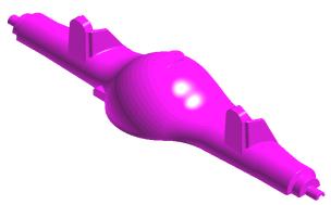
(a) Curve-nets given (b) Mesh surface generated

Fig.9. Rear axle surface generation

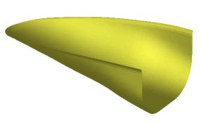
(a) Curve-nets given (b) Mesh surface generated

Fig.10. Aerodynamic Fairing surface generation

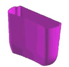
(a) Curve-net given (b) Mesh surface generated

Fig.10. Water tank surface generation

References

[1] Konno K. And Chiyokura H., A approach of designing and controlling free-form surfaces by using NURBS boundary Gregory patches, Computer aided geometric design, Vol.13, 1996, pp.825-849.

[2] Gregory J.A., Smooth interpolation without twist constrains, Computer Aided Geometric Design, Academic-Press, 1974, pp.27-33.

[3] Chiyokura H., Takamura T., Konno K., Harada T., surface interpolation over irregular meshes with rational curves. In: Farin G., ed., NURBS for curves and surfaces design, SIAM, Philadelphia PA, 1991, pp.15-34.

[4] Piegl,L. and Tiller,W., The NURBS Book, Springer, 1995.

[5] Toriya H. And Chiyokura H., eds., 3D CAD Principles and Application, Springer, 1993.